ML in ClickHouse

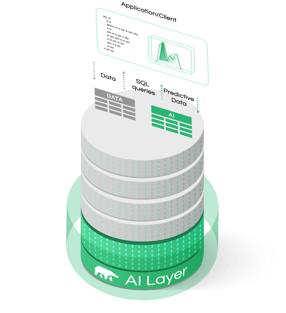
In previous blog posts, we examined the importance of housing your machine learning applications at the data layer. There are many similarities in the features and structures of both databases and machine learning applications which are conducive to applying machine learning directly at the data source. It saves time, allows you to quickly operationalize machine learning, and reduces both data wrangling and the Extract-Transform-Loading (ETL) of data. By allowing the application layer to query predictions in the same way as it queries actual data, you can seamlessly introduce machine learning into your business applications.

Time-Series is Hard

One of the fastest-growing sets of use cases today is forecasting over structured data, but at the same, sometimes it becomes a very difficult machine learning problem even for most data scientists.

For instance, the most important component of the use cases we explored for this type of data was multivariate time series, which present particular challenges in data science.

Take the industrial sensor example – if you wanted to predict machine failure or maintenance requirements, you would likely be dealing with thousands of sensors. Each sensor (at each industrial facility) would have its own set of time stamps. This would mean many thousands of individual time series which normally would each require a machine learning model to be trained and launched in production.

In today’s post, we would like to dive a bit deeper into the challenges of time series, and explore another use case for high-performance analytics on large data sets (and time series) using Clickhouse.

Clickhouse for Analytics

Clickhouse is a column-oriented Database Management System (DBMS) that is particularly well suited for Online Analytical Processing (OLAP). While Clickhouse doesn’t support transactions, and things like INSERT statements are relatively slow and best handled in batch, queries involving a large number of rows (and often a subset of columns) are lightning fast. The columnar nature of Clickhouse makes it ideal for multi-dimensional analysis and analysis of data sets with a high degree of cardinality. Time series often fall into both of the two aforementioned categories. Thus, if you want to quickly analyze a large time series, it can be done efficiently in Clickhouse. Similarly, if you want to build a predictive machine-learning model for a large, multivariate time series, Clickhouse is again a great choice.

Time-Series are even Harder Than We Thought...

Time series often present a high degree of cardinality - meaning that in one single table, rows can belong to an enormous number of groups. Imagine a table that contains all transactions in a very large store that sells thousands of products, and suppose that each row in this table contains the following information: transaction time, product, quantity, customer ID. If you want to forecast demand for all products given the information of this table, you will need to organize and group rows by product, meaning that in this table you will have as many groups of transactions as products. Let’s consider a set of New York City taxi data that contains millions of individual rows identified by a timestamp. It has columns for fare price, ride distance, passenger number, and potentially dozens of other features. Notably, these features are interrelated in subtle ways and they influence one another over long time horizons. For example, fare prices vary depending on the time of day. Passenger numbers also fluctuate as they are likely to be lower in the morning when people are commuting. Other features may be purely stochastic. Lastly, some features might be subject to a random walk over long periods and then find themselves influenced by other features during certain periods. You may ask yourself, “Isn’t this what Long Short Term Memory networks are designed for?” (LSTMs are a type of recurrent neural network that often deal well with long time horizons). LSTM predictions are hard to explain, and their performance often falls behind predictions using simple lagged values when it comes to large, multivariate time series. In addition, LSTMs that are applied to long, relatively stochastic periods might produce predictions with a deceptively accurate fit to actual data. In reality, they might simply be predicting a value at t+1 using the value at t. In fact, the R2 score may look great for a particular time interval but it is not necessarily helpful in determining the overall accuracy of the model.

Adaptive Models and Mixers Work

Practice has shown that a combination of adaptive models can work extremely well for exactly this sort of problem. MindsDB uses a gradient booster mixer (based on LightGBM) and a feedforward neural network mixer. A mixer combines the intermediate representations of encoders to achieve the performance of larger, more complex models. It is an ML model that takes as input the features of all pre-trained encoders and learns to predict the encoded representation of the target column(s). Rather than combining the architectures of the encoders themselves, it uses their outputs. Our research into combined, adaptive models parallels other teams (particularly at Google) that demonstrate that a mixer merging relatively simple feed-forward Neural Network (NN) architectures competes well with larger CNN models.

The LightGBM and NnMixer are complementary in the sense that at least one of them performs nicely for a typical predictive task. However, at the end of the model selection phase only one of them is saved as the predictor.

If you would like to see how this works, please watch our Webinar recording! We did a walkthrough of interesting use cases and generated accurate predictions on large time-series with Clickhouse and MindsDB.

‍